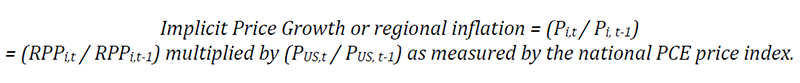
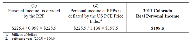
Today, the U.S. Bureau of Economic Analysis released experimental real, or inflation-adjusted, estimates of personal income for states and metropolitan areas. The inflation-adjustments are based in part on regional price parities (RPPs) that provide a measure of differences in price levels across each state and region relative to the national price level for each of the years, 2007-2011. When RPPs are applied in conjunction with BEA’s national Personal Consumption Expenditures (PCE) price index, which measures price changes over time, personal income comparisons can be made across regions and time periods (see Technical Note). These prototype statistics are being released for evaluation and comment by data users.

Real Personal Income for States and Metropolitan Areas¹

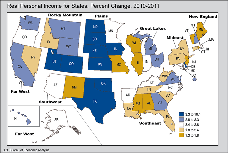
Real personal income across all regions rose by an average of 2.7% in 2011, after rising 1.9% in 2010. These growth rates reflect the year-over-year change in nominal personal income across all regions adjusted by the change in the national PCE price index. On a nominal basis, personal income across all regions grew an average of 5.2% in 2011, after rising 3.8% in 2010. In 2011, the U.S. PCE price index grew 2.4% after rising 1.9% in 2010.

Growth in real state personal income from 2010 to 2011 ranged from 1.3% in Mississippi to 10.4% in South Dakota. These growth rates reflect the year-over-year change in the state’s nominal personal income, the change in the national PCE price index, and the change in the regional price parity for that state. After South Dakota, the states with the largest growth rates of real personal income are North Dakota (9.5%), Iowa (6.1%), Nebraska (6.0%), and Texas (4.3%). The states with smallest growth rates after Mississippi are Maine (1.4%), Rhode Island (1.5%), Vermont (1.6%), and New Mexico (1.6%). Four states – Arizona, Indiana, North Carolina, and Oregon – had growth rates equal to the national average of 2.7%.

Growth in real metropolitan area personal income from 2010 to 2011 ranged from a decline of 0.7% in Rochester, MN to an increase of 11.9% in Odessa, TX. After Odessa, TX, the metropolitan areas with largest growth rates of real personal income were Midland, TX (10.7%), Hanford-Corcoran, CA (6.7%), San Jose-Sunnyvale-Santa Clara, CA (6.4%), and Madera-Chowchilla, CA (6.2%). In addition to Rochester, MN, four metropolitan areas had declining or flat growth rates. These are Ocean City, NJ (-0.3%), Anniston-Oxford, AL (-0.2%), Gadsden, AL (-0.2%), and Cape Girardeau-Jackson, MO-IL (0.0%).

Regional Price Parities

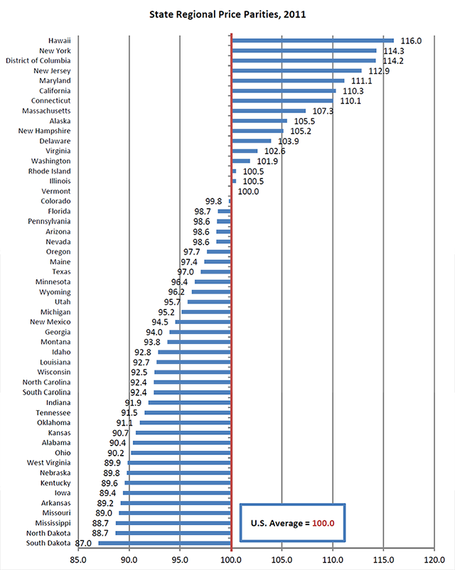
Regional Price Parities (RPPs) measure the differences in the price levels of goods and services across states and metropolitan areas for a given year. RPPs are expressed as a percentage of the overall national price level for each year, which is equal to 100.0.

In 2011, the states with the highest RPPs were Hawaii (116.0), New York (114.3), and the District of Columbia (114.2). High RPPs in these states were driven by the relatively high price level of rents and other services. South Dakota (87.0), North Dakota (88.7), and Mississippi (88.7) had the lowest RPPs among the States. States with low RPPs typically have lower price levels for rents and other services, while the price level for goods is relatively higher. States with RPPs close or equal to the national average price level were Colorado (99.8), Illinois (100.5), Rhode Island (100.5), and Vermont (100.0).

In 2011, the metropolitan area with the highest RPP was Bridgeport-Stamford-Norwalk, CT (122.3). Metropolitan areas with RPPs above 120.0 also include Honolulu, HI (121.0), Poughkeepsie-Newburgh-Middletown, NY (120.6), and New York-Northern New Jersey-Long Island, NY-NJ-PA (120.5). The metropolitan area with lowest RPP was Jefferson City, MO (81.0), followed by Morristown, TN (82.3), Danville, IL (82.5), and Cape Girardeau-Jackson, MO-IL (82.9).

Technical Note on Real Personal Income for States and Metropolitan Areas

Price indexes commonly measure price changes over time. The BEA’s Personal Consumption Expenditure price index and the BLS’ Consumer Price Index are two examples. Spatial price indexes measure price level differences across regions for one time period. An example of these latter type of indexes are purchasing power parities (PPPs), which measure differences in price levels across countries for a given period, and can be used to convert estimates of per capita GDP into comparable levels in a common currency. RPPs similarly compare regions within the United States, but without the need for currency conversion.

The RPPs are calculated using price quotes for a wide array of items from the CPI, which are then aggregated into broader expenditure categories (such as food, transportation, or education) to obtain relative price levels for each area. Data on rents are obtained separately from the Census Bureau’s American Community Survey. The expenditure weights for each category are constructed using the BLS’ Consumer Expenditure Survey and BEA’s Personal Consumption Expenditures. The RPP indexes are calculated using the Geary² system and express a region’s average price relative to the US average, which is equal to 100.0. That is,

The real personal income statistics presented in this release use the national PCE price index to measure US price change over time and RPPs to capture the change in price level differences over time across states. The implicit price growth for each state can be calculated as,

For example, if the RPP for area A is 120 and for area B is 90, then on average, prices are 20% higher and 10% lower than the US average for A and B respectively. If the Personal Income for area A is $12,000 and for area B is $9,000, then RPP-adjusted incomes are $10,000 ($12,000/1.20) and $10,000 ($9,000/0.90) respectively. In other words, the purchasing power of the two incomes is equivalent when adjusted by their respective area price levels.

This release includes annual RPPs for the years 2007 through 2011. These are based on annual price levels for the rents category and five-year rolling average price levels for all other categories. We use five-year averages for the price levels of goods and services other than rents to improve the stability of the underlying estimates based on the CPI sample. The expenditure weights are specific to each year. Detailed information on the methodology used to estimate the RPPs may be found in a forthcoming article in the August 2013 issue of the Survey of Current Business.

Definitions

Personal income is the income received by all persons from all sources. Personal income is the sum of net earnings by place of residence, property income, and personal current transfer receipts. These are current dollar estimates. Comparisons for different regions and time periods reflect changes in both the price and quantity components of regional personal income.

Estimates of personal income in the United States are derived as the sum of the regional estimates. These differ from the estimates of personal income in the national income and product account (NIPAs) because of differences in coverage, in the methodologies used to prepare the estimates, and in the timing of the availability of source data.

Regional price parities (RPPs) are regional price levels expressed as a percentage of the overall national price level for a given year. The price level is determined by the average prices paid by consumers for the mix of goods and services consumed in each region. The RPPs are calculated using data from the Bureau of Labor Statistics’ (BLS) Consumer Price Index (CPI) program and the Census Bureau’s American Community Survey (ACS).

Detailed CPI price data are adjusted to obtain average price levels for BLS-defined areas³. These are allocated to counties in combination with direct price and expenditure data on rents from the ACS. County data are then aggregated to states and metropolitan areas.

Personal income at RPPs is current-dollar personal income divided by the price parity⁴ for a given year and region (state, state metropolitan and non-metropolitan portions, or metropolitan area).

Real personal income is the personal income at RPPs divided by the national PCE chain-type price index. The result is a real personal income estimate in chained dollars (using 2005 as the reference year). Using Colorado in 2011 as an example:

Estimates of real personal income in the United States are derived as the sum of the regional estimates divided by the U.S. PCE Price Index.

Next Steps

BEA plans outreach with data users to assess these prototype estimates. Subject to data users’ evaluations and comments, we plan to monitor revisions to these estimates, to review the methodology, and to look at methods for accelerating the release of these estimates. Provided user evaluations are positive, our plan for 2014 is to release new estimates, incoporating feedback that will improve the accuracy, consistency, and relevance of the estimates.

These data are prototype statistics in that they are being released for evaluation and comment by data users. There has been substantial interest in these statistics, and BEA hopes to produce real state and metropolitan area personal income as annual series in the future. If you have comments or suggestions, please send these to rpp@bea.gov.

* * *

The state tables in this press release are also available on the BEA website. Additional tables showing estimates of real income and regional price parities can also be found there for:

• State metropolitan and non-metropolitan portions, 2007-2011
• Metropolitan areas, 2009-2011

BEA’s national, international, regional, and industry statistics; the Survey of Current Business; and BEA news releases are available without charge on BEA’s web site at www.bea.gov. By visiting the site, you can also subscribe to receive free e-mail summaries of BEA releases and announcements.

Next real personal income release – June 2014 for states, state metropolitan and nonmetropolitan portions, and metropolitan areas.