Today, the U.S. Bureau of Economic Analysis released real, price-adjusted estimates of personal income for states and metropolitan areas for 2008-2012.

"For the first time, Americans looking to move or take a job anywhere in the country can compare inflation-adjusted incomes across states and metropolitan areas to better understand how their personal income may be affected by a job change or move. Businesses considering relocating or establishing new plants also now have a comprehensive and consistent measure of differences in the cost of living and the purchasing power of consumers nationwide. The Commerce Department’s 'Open for Business Agenda' prioritizes making our data more accessible and understandable so that it can continue powering both small and large businesses nationwide," said U.S. Secretary of Commerce Penny Pritzker.

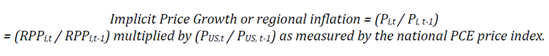
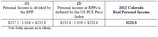
The price-adjustments are based on regional price parities (RPPs) and on BEA’s national Personal Consumption Expenditure (PCE) price index. The RPPs measure geographic differences in the price levels of consumption goods and services relative to the national average, and the PCE price index measures national price changes over time (see Technical Note). Using the RPPs in combination with the PCE price index allows for comparisons of the purchasing power of personal income across regions and over time. These estimates are being released for the first time as official statistics¹.

Real Personal Income for States and Metropolitan Areas

Real personal income across all regions rose by an average of 2.3% in 2012. This growth rate reflects the year-over-year change in nominal personal income across all regions adjusted by the change in the national PCE price index. On a nominal basis, personal income across all regions grew an average of 4.2% in 2012. In 2012, the U.S. PCE price index grew 1.8%.

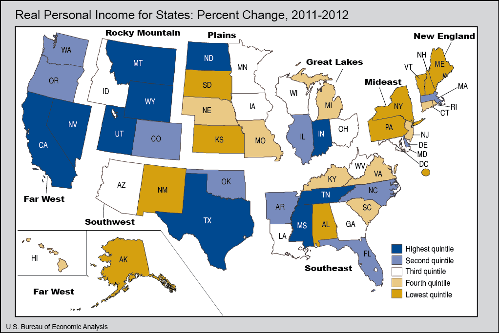
Growth in real state personal income from 2011 to 2012 ranged from a decline of 1.2% in South Dakota to an increase of 15.1% in North Dakota. These growth rates reflect the year-over-year change in the state’s nominal personal income, the change in the national PCE price index, and the change in the regional price parity for that state. After North Dakota, the states with the largest growth rates were Montana (3.7%), Indiana (3.7%), California (3.4%), and Mississippi (3.4%). South Dakota was the only state with a decline in real personal income. The states with the smallest growth rates were Maine (0.3%), Alaska (0.7%), and Alabama (0.8%). The District of Columbia’s growth rate was 0.4%. States with growth rates close to the national average were Delaware (2.4%), Georgia (2.2%), Illinois (2.4%), Minnesota (2.2%), and Oregon (2.4%).

Growth in real metropolitan area personal income from 2011 to 2012 ranged from a decline of 3.8% in Kennewick-Richland, WA to an increase of 10.2% in Odessa, TX. After Odessa, TX, the metropolitan areas with the largest growth rates were Midland, TX (9.6%), Greenville, NC (9.0%), Jackson, TN (8.1%), and Columbus, IN (7.6%). After Kennewick-Richland, WA, the metropolitan areas with the largest declines were Watertown-Fort Drum, NY (-2.5%), State College, PA (-2.4%), Hanford-Corcoran, CA (-2.3%), and Sierra Vista-Douglas, AZ (-1.7%).

Regional Price Parities

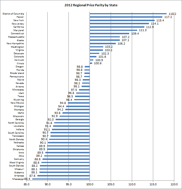
Regional Price Parities (RPPs) measure the differences in the price levels of goods and services across states and metropolitan areas for a given year. RPPs are expressed as a percentage of the overall national price level for each year, which is equal to 100.0.

In 2012, the District of Columbia’s RPP (118.2) was higher than that of any state. The states with the highest RPPs were Hawaii (117.2), New York (115.4), New Jersey (114.1), and California (112.9). Mississippi (86.4), Arkansas (87.6), Alabama (88.1), Missouri (88.1), and South Dakota (88.2) had the lowest RPPs among the States. States with high (low) RPPs typically have relatively high (low) price levels for rents. States with RPPs closest to the national average price level were Florida (98.8), Oregon (98.8), Illinois (100.6), and Vermont (100.9).

In 2012, the metropolitan area with the highest RPP was Urban Honolulu, HI (122.9). Metropolitan areas with RPPs above 120.0 also include New York-Newark-Jersey City, NY-NJ-PA (122.2), San Jose-Sunnyvale-Santa Clara, CA (122.0), Bridgeport-Stamford-Norwalk, CT (121.5), Santa Cruz-Watsonville, CA (121.4), San Francisco-Oakland-Hayward, CA (121.3), and Washington-Arlington-Alexandria, DC-VA-MD-WV (120.4). The metropolitan area with lowest RPP was Danville, IL (79.4), followed by Jefferson City, MO (80.8), Jackson, TN (81.5), Jonesboro, AR (81.7), and Rome, GA (82.2).

Technical Note on Regional Price Parities and Implicit Regional Price Deflators

Price indexes commonly measure price changes over time. The BEA’s Personal Consumption Expenditure price index and the BLS’ Consumer Price Index (CPI) are two examples. Spatial price indexes measure price level differences across regions for one time period. An example of these type of indexes are purchasing power parities (PPPs), which measure differences in price levels across countries for a given period, and can be used to convert estimates of per capita GDP into comparable levels in a common currency. The regional price parities (RPPs) that BEA has developed compare regions within the United States, but without the need for currency conversion. An implicit regional price deflator (IRPD) can be derived by combining the RPPs and the PCE price index.

Regional Price Parities. The RPPs are calculated using price quotes for a wide array of items from the CPI, which are aggregated into broader expenditure categories (such as food, transportation, or education). Data on rents are obtained separately from the Census Bureau’s American Community Survey (ACS). The expenditure weights for each category are constructed using the BLS’ Consumer Expenditure Survey and BEA’s Personal Consumption Expenditures².