
News Release
Real Personal Income for States and Metropolitan Areas, 2015
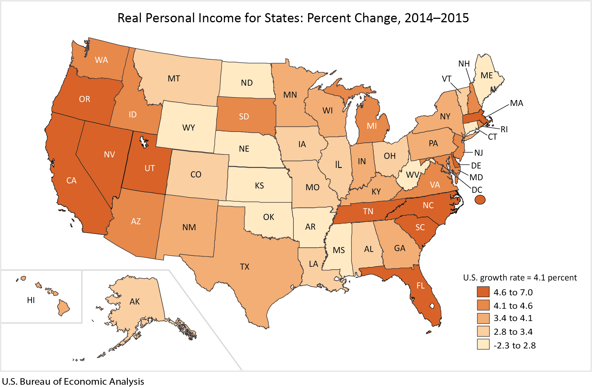
Real state personal income grew on average 4.1 percent in 2015, after increasing 3.6 percent in 2014, according to estimates released today by the Bureau of Economic Analysis. Growth of real state personal income – a state's current-dollar personal income adjusted by the state's regional price parity and the national personal consumption expenditure price index – ranged from -2.3 percent in North Dakota to 7.0 percent in Delaware (table 1). Across metropolitan areas, growth ranged from -10.1 percent in Midland, TX to 9.9 percent in Carson City, NV (table 4).
Real Personal Income Growth Rates
- States with the fastest growth in real personal income were Delaware (7.0 percent), Oregon (6.1 percent), and California (6.1 percent). The District of Columbia's real personal income grew 6.6 percent.
- The only state with declining real personal income was North Dakota (-2.3 percent). States with the slowest growth in real personal income were Wyoming (0.5 percent), Nebraska (0.7 percent), and Oklahoma (1.3 percent).
- Large metropolitan areas – those with population greater than two million – with the fastest growth in real personal income were San Francisco-Oakland-Hayward, CA (7.4 percent), Orlando-Kissimmee-Sanford, FL (6.5 percent), Riverside-San Bernardino-Ontario, CA (6.4 percent), and Sacramento--Roseville--Arden-Arcade, CA (6.4 percent).
- Large metropolitan areas with the slowest growth in real personal income were Cleveland-Elyria, OH (2.8 percent), Denver-Aurora-Lakewood, CO (2.8 percent), and Cincinnati, OH-KY-IN (3.0 percent).
Regional Price Parities
Regional Price Parities (RPPs) measure the differences in price levels across states and metropolitan areas for a given year and are expressed as a percentage of the overall national price level. All items RPPs cover all consumption goods and services, including rents. Areas with high/low all items RPPs typically correspond to areas with high/low price levels for rents.
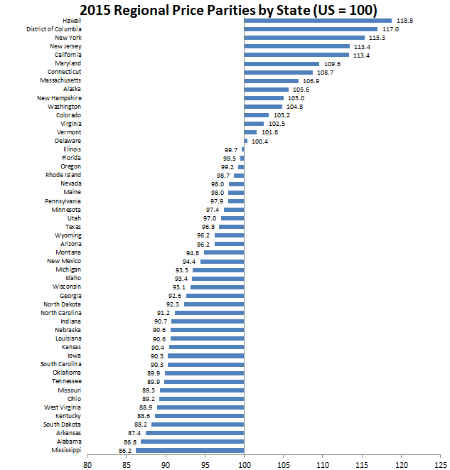
- States with the highest all items RPPs were Hawaii (118.8), New York (115.3), New Jersey (113.4), and California (113.4) (table 3). The District of Columbia's RPP was 117.0.
- States with the lowest all items RPPs were Mississippi (86.2), Alabama (86.8), and Arkansas (87.4).
- Across states, Hawaii had the highest rents RPP (163.4) and Alabama had the lowest (62.8).
- Large metropolitan areas with the highest all items RPP were New York-Newark-Jersey City, NY-NJ-PA (121.9), San Francisco-Oakland-Hayward, CA (121.9), and Washington-Arlington-Alexandria, DC-VA-MD-WV, (119.1) (table 6).
- Large metropolitan areas with the lowest all items RPP were Cincinnati, OH-KY-IN (89.2), Cleveland-Elyria, OH (89.7), and St. Louis, MO-IL (90.6).
- Across large metropolitan areas, San Francisco-Oakland-Hayward, CA had the highest rents RPP (186.0) and Cleveland-Elyria, OH had the lowest (78.7).
Next release: June 2018 — Real Personal Income for States and Metropolitan Areas, 2016
Estimates of real personal income and regional price parities for state metropolitan and nonmetropolitan portions, and metropolitan areas can be found at https://www.bea.gov/itable. Supplemental tables are available upon request.
Technical Notes on Regional Price Parities and Implicit Regional Price Deflators
Price indexes commonly measure price changes over time. The BEA's personal consumption expenditure (PCE) price index and the Bureau of Labor Statistics' consumer price index (CPI) are two examples. Spatial price indexes measure price level differences across regions for one time period. An example of these type of indexes are purchasing power parities (PPPs), which measure differences in price levels across countries for a given period, and can be used to convert estimates of per capita GDP into comparable levels in a common currency. The regional price parities (RPPs) that BEA has developed compare regions within the United States, but without the need for currency conversion. An implicit regional price deflator (IRPD) can be derived by combining the RPPs and the U.S. PCE price index.
Regional Price Parities. The RPPs are calculated using price quotes for a wide array of items from the CPI, which are aggregated into broader expenditure categories (such as food, transportation or education) . Data on rents are obtained separately from the Census Bureau's American Community Survey (ACS). The expenditure weights for each category are constructed using CPI expenditure weights, BEA's personal consumption expenditures, and ACS rents expenditures2.
The broader categories and the data on rents are combined with the expenditure weights using a multilateral aggregation method that expresses a region's price level relative to the U.S.3
For example, if the RPP for area A is 120 and for area B is 90, then on average, prices are 20 percent higher and 10 percent lower than the U.S. average for A and B, respectively. If the personal income for area A is $12,000 and for area B is $9,000, then RPP-adjusted incomes are $10,000 (or $12,000/1.20) and $10,000 (or $9,000/0.90), respectively. In other words, the purchasing power of the two incomes is equivalent when adjusted by their respective RPPs.
Implicit Regional Price Deflator. The IRPD is a regional price index derived as the product of two terms: the regional price parity and the U.S. PCE price index.
The implicit regional price deflator will equal current dollar personal income divided by real personal income in chained dollars. The growth rate or year-to-year change in the IRPDs is a measure of regional inflation4.
Detailed information on the methodology used to estimate the RPPs may be found on the regional methodology page of the BEA website:www.bea.gov/regional/methods.cfm.
BEA's national, international, regional, and industry statistics; the Survey of Current Business; and BEA news releases are available without charge on BEA's website at www.bea.gov. By visiting the site, you can also subscribe to receive free e-mail summaries of BEA releases and announcements.
Definitions
Personal income is the income received by all persons from all sources. Personal income is the sum of net earnings by place of residence, property income, and personal current transfer receipts. These are current dollar estimates. Comparisons for different regions and time periods reflect changes in both the price and quantity components of regional personal income.
Estimates of personal income in the United States are derived as the sum of the regional estimates. These differ from the estimates of personal income in the national income and product accounts (NIPAs) because of differences in coverage, in the methodologies used to prepare the estimates, and in the timing of the availability of source data.
Regional price parities (RPPs) are regional price levels expressed as a percentage of the overall national price level for a given year. The price level is determined by the average prices paid by consumers for the mix of goods and services consumed in each region.
Detailed CPI price data are adjusted to obtain average price levels for BLS-defined areas5. These are allocated to counties in combination with direct price and expenditure data on rents from the ACS.
County data are then aggregated to states and metropolitan areas.
Personal income at RPPs is current-dollar personal income divided by the price parity6 for a given year and region. A balancing factor is applied so that the sum of personal income at RPPs across regions equals the current dollar sum.
Real personal income is personal income at RPPs divided by the national PCE chain-type price index. The result is real personal income in chained dollars (using 2009 as the reference year). Using Alaska in 2015 as an example:
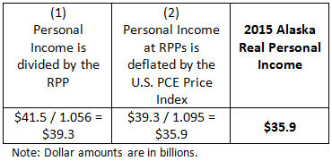
Estimates of real personal income in the United States are derived as the sum of the regional estimates divided by the U.S. PCE Price Index.
Implicit Regional Price Deflator (IRPD) is the product of the RPP times the national PCE price index. It is equal to personal income divided by real personal income. See also the Technical Note.
1 The BEA Regional Price Parity statistics are based in part on restricted access Consumer Price Index data from the Bureau of Labor Statistics (BLS). The BEA statistics presented herein are products of BEA and not BLS.
2 To estimate RPPs, CPI price quotes are quality adjusted and pooled over 5 years. The ACS rents are also quality adjusted and are either annual for states or pooled over 3 years for metropolitan areas. The expenditure weights are specific for each year.
3 The multilateral system that is used is the Geary additive method. Any region or combination of regions may be used as the base or reference region without loss of consistency.
4 The growth rate of the implicit regional price deflators will not necessarily equal the region or metro area price deflators published by the BLS. This is because the CPI deflators are calculated directly while the IRPDs are indirect estimates, and because of differences in the source data and methodology.
5 The CPI represents about 89 percent of the total U.S. population, including almost all residents of urban or metropolitan areas. In the northeast region, rural area prices (exclusive of rents) are assumed to be the same as those in the small metropolitan areas of the CPI; in the midwest, south, and west regions, they are assumed to be the same as those in the nonmetropolitan urban areas of the CPI.
6 RPP should first be divided by 100.