
News Release
Real Personal Income by State and Metropolitan Area, 2019
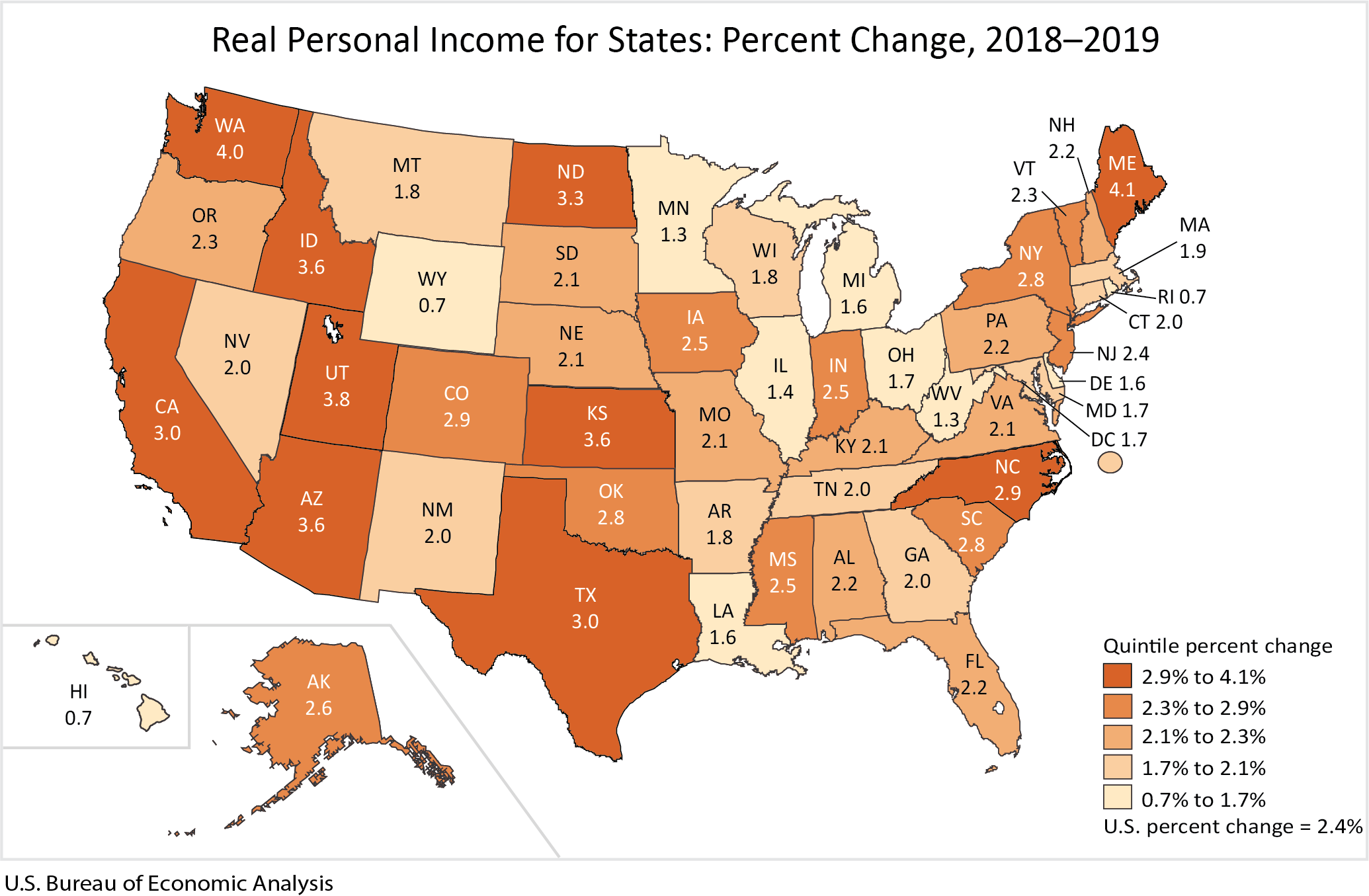
Real state personal income grew 2.4 percent in 2019 after increasing 3.1 percent in 2018, according to estimates released today by the Bureau of Economic Analysis (BEA). Real state personal income is a state's current-dollar personal income adjusted by the state's regional price parity and the national personal consumption expenditures price index. The percent change in real state personal income ranged from 4.1 percent in Maine to 0.7 percent in Hawaii, Wyoming, and Rhode Island (table 1). Across metropolitan areas, the percent change ranged from 7.6 percent in Hanford-Corcoran, CA, to –3.2 percent in Panama City, FL, and Wheeling, WV-OH (table 4).
Real Personal Income in 2019
- States with the fastest growth in real personal income were Maine (4.1 percent), Washington (4.0 percent), and Utah (3.8 percent).
- No state had a decline in real personal income. States with the slowest growth in real personal income were Rhode Island (0.7 percent), Wyoming (0.7 percent), and Hawaii (0.7 percent).
- Large metropolitan areas—those with populations greater than two million—with the fastest growth in real personal income were Austin-Round Rock-Georgetown, TX (5.3 percent), Denver-Aurora-Lakewood, CO (4.0 percent), and Riverside-San Bernardino-Ontario, CA (3.7 percent).
- Large metropolitan areas with the slowest growth in real personal income were Miami-Fort Lauderdale-Pompano Beach, FL (1.4 percent), Chicago-Naperville-Elgin, IL-IN-WI (1.4 percent), and Detroit-Warren-Dearborn, MI (1.4 percent).
Regional Price Parities in 2019
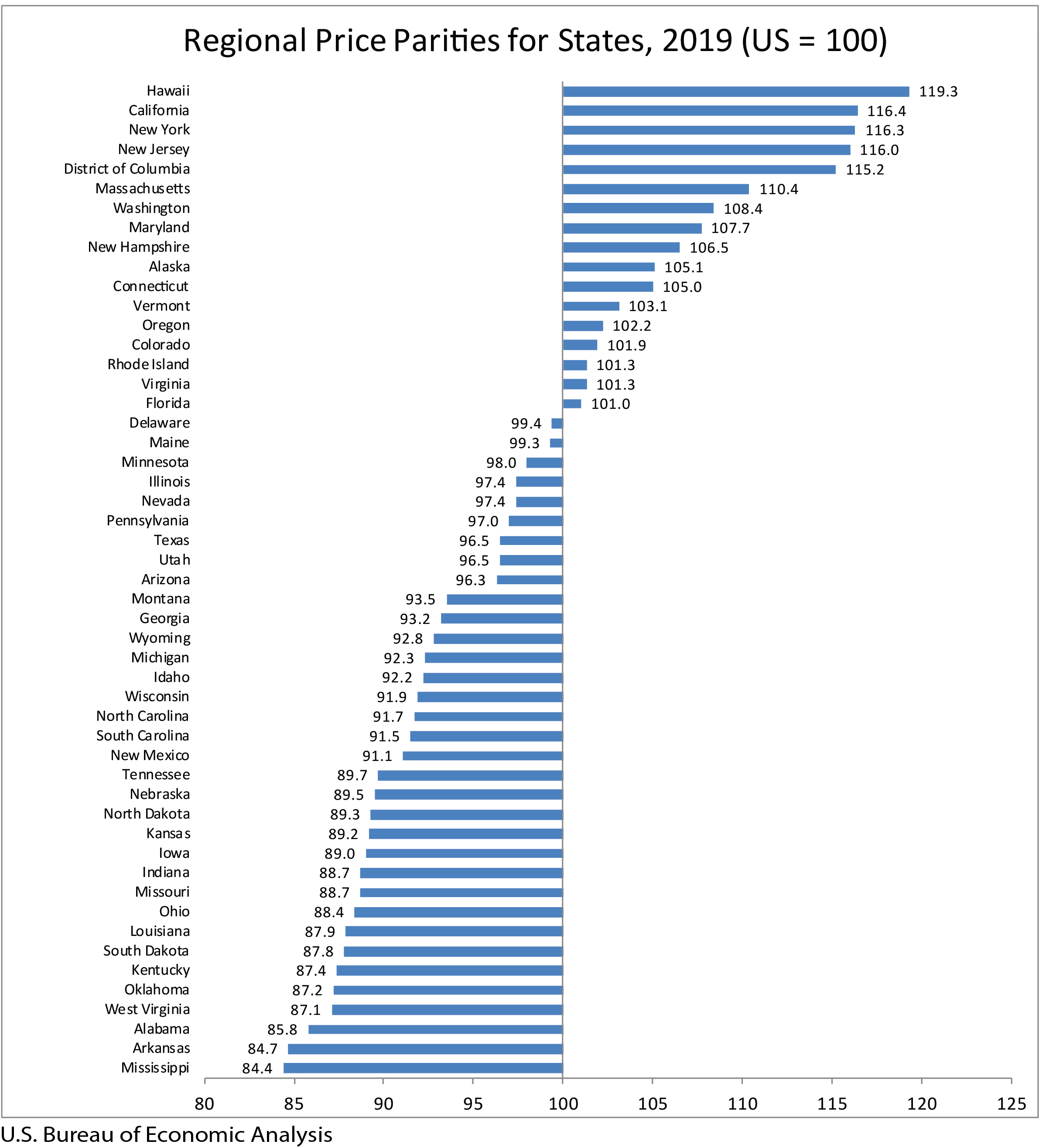
Regional price parities (RPPs) measure the differences in price levels across states and metropolitan areas for a given year and are expressed as a percentage of the overall national price level. The all items RPP covers all consumption goods and services, including housing rents. Areas with high/low RPPs typically correspond to areas with high/low price levels for rents.
- States with the highest RPPs were Hawaii (119.3), California (116.4), and New York (116.3) (table 3).
- States with the lowest RPPs were Mississippi (84.4), Arkansas (84.7), and Alabama (85.8).
- Across states, California had the highest RPP for housing rents (153.6), and Mississippi had the lowest (60.0).
- Large metropolitan areas with the highest RPPs were San Francisco-Oakland-Berkeley, CA (134.5), New York-Newark-Jersey City, NY-NJ-PA (125.7), and Los Angeles-Long Beach-Anaheim, CA (118.8) (table 6).
- Large metropolitan areas with the lowest RPPs were Cleveland-Elyria, OH (89.9), St. Louis, MO-IL (90.1), and Cincinnati, OH-KY-IN (90.6).
- Across large metropolitan areas, San Francisco-Oakland-Berkeley, CA, had the highest RPP for housing rents (200.3), and Cleveland-Elyria, OH, had the lowest (76.3).
- Across all metropolitan areas, San Jose-Sunnyvale-Santa Clara, CA, had the highest RPP for housing rents (224.0), and Beckley, WV, had the lowest (44.0).
Estimates of real personal income and regional price parities for state metropolitan and nonmetropolitan portions can be found at https://apps.bea.gov/itable/index.cfm. Supplemental tables are available upon request.
Acceleration of Release of Real Personal Income by State and Metropolitan Area
Today's release of real personal income by state and metropolitan area for 2019 represents a 5-month acceleration in the release of these statistics relative to last year's release schedule.
Annual Update of Real Personal Income
The estimates of 2019 state and metropolitan area real personal income released today incorporate the results of BEA's annual update of state and metropolitan area real personal income, also released today. The annual estimates for 2017 and 2018 were revised. The update incorporates revised source data that are more complete and more detailed than previously available.
Release of Real Personal Consumption Expenditures by State
On December 14, 2021, BEA will for the first time release official statistics of real personal consumption expenditures. These data will be combined with statistics on real personal income by state and metropolitan area in a single release for 2020.
Next release: December 14, 2021, at 8:30 A.M. EST
Real Personal Consumption Expenditures by State and
Real Personal Income by State and Metropolitan Area, 2020
* * *
Technical Notes on Regional Price Parities and Implicit Regional Price Deflators
Price indexes commonly measure price changes over time. The BEA personal consumption expenditures (PCE) price index and the Bureau of Labor Statistics (BLS) Consumer Price Index (CPI) are two examples. Spatial price indexes measure price level differences across regions for one time period. An example of this type of index is purchasing power parities (PPPs), which measure differences in price levels across countries for a given period, and can be used to convert estimates of per capita gross domestic product into comparable levels in a common currency. The RPPs that BEA has developed compare regions within the United States but without the need for currency conversion. An implicit regional price deflator (IRPD) can be derived by combining the RPPs and the U.S. PCE price index.
Regional price parities. The RPPs are calculated using price quotes for an array of items from the CPI, which are aggregated into broader expenditure categories (such as food, transportation, or education).1 Data on rents are obtained separately from the Census Bureau American Community Survey (ACS). The expenditure weights for each category are constructed using CPI expenditure weights, BEA personal consumption expenditures, and ACS rents expenditures.2
The broader categories and the data on rents are combined with the expenditure weights using a multilateral aggregation method that expresses a region's price level relative to the United States.3
For example, if the RPP for area A is 120 and the RPP for area B is 90, then on average, prices are 20 percent higher and 10 percent lower than the U.S. average for A and B, respectively. If the personal income for area A is $12,000 and the personal income for area B is $9,000, then RPP-adjusted incomes are $10,000 (or $12,000/1.20) and $10,000 (or $9,000/0.90) for A and B, respectively. In other words, the purchasing power of the two incomes is equivalent when adjusted by their respective RPPs.
Implicit regional price deflator. The IRPD is a regional price index derived as the product of two terms: the regional price parity and the U.S. PCE price index.
The implicit regional price deflator will equal current-dollar personal income divided by real personal income in chained dollars. The growth rate, or year-to-year change, in the IRPDs is a measure of regional inflation.4
Detailed information on the methodology used to estimate RPPs may be found on the regional methodology page of the BEA website: https://www.bea.gov/regional/methods.cfm.
1 The BEA Regional Price Parity statistics are based in part on restricted access Consumer Price Index data from the Bureau of Labor Statistics (BLS). The BEA statistics presented herein are products of BEA and not BLS.
2 To estimate RPPs, CPI price quotes are quality adjusted and pooled over 5 years. The ACS rents are also quality adjusted and are either annual for states or pooled over 3 years for metropolitan areas. The expenditure weights are specific for each year.
3 The multilateral system that is used is the Geary additive method. Any region or combination of regions may be used as the base or reference region without loss of consistency.
4 The growth rate of the implicit regional price deflators will not necessarily equal the region or metro area price deflators published by the BLS. This is because the CPI deflators are calculated directly while the IRPDs are indirect estimates, and because of differences in the source data and methodology.
Resources
- Stay informed about BEA developments by reading The BEA Wire, signing up for BEA's email subscription service, or following BEA on Twitter @BEA_News.
- Historical time series for these estimates can be accessed in BEA's Interactive Data Application.
- Access BEA data by registering for BEA's Data Application Programming Interface (API).
- For more on BEA's statistics, see our monthly online journal, the Survey of Current Business.
- BEA's news release schedule.
Definitions
Personal income is the income received by, or on behalf of, all persons from all sources—from participation as laborers in production, from owning a home or business, from the ownership of financial assets, and from government and business in the form of transfers. It includes income from domestic sources as well as the rest of world. It does not include realized or unrealized capital gains or losses.
Personal income is measured before the deduction of personal income taxes and other personal taxes and is reported in current dollars (no adjustment is made for price changes). Comparisons for different regions and time periods reflect changes in both the price and quantity components of regional personal income.
The estimate of personal income for the United States is the sum of the state estimates and the estimate for the District of Columbia; it differs slightly from the estimate of personal income in the National Income and Product Accounts because of differences in coverage, in the methodologies used to prepare the estimates, and in the timing of the availability of source data.
Per capita personal income is calculated as the total personal income of the residents of a given area divided by the population of the area. In computing per capita personal income, BEA uses Census Bureau midyear population estimates.
Regional price parities are regional price levels expressed as a percentage of the overall national price level for a given year. The price level is determined by the average prices paid by consumers for the mix of goods and services consumed in each region.
Detailed CPI price data are adjusted to obtain average price levels for BLS-defined areas5. These are allocated to counties in combination with direct price and expenditure data on rents from the ACS. County data are then aggregated to states and metropolitan areas.
Personal income at RPPs is current-dollar personal income divided by the price parity6 for a given year and region. A balancing factor is applied so that the sum of personal income at RPPs across regions equals the current-dollar sum.
Real personal income is personal income at RPPs divided by the national PCE chain-type price index. The result is real personal income in chained dollars (using 2012 as the reference year). Using Montana in 2019 as an example:
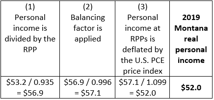
Note. Dollar amounts are in billions.
Estimates of real personal income in the United States are derived as the sum of the regional estimates divided by the U.S. PCE price index.
Implicit regional price deflator is the product of the RPP times the national PCE price index. It is equal to personal income divided by real personal income. See also the "Technical Note."
5 The CPI represents about 93 percent of the total U.S. population, including almost all residents of urban or metropolitan areas.
6 RPP should first be divided by 100.
List of News Release Tables
Table 1. Real Personal Income and Implicit Regional Price Deflators by State, 2018–2019
Table 2. Real Per Capita Personal Income by State, 2018–2019
Table 3. Regional Price Parities by State, 2019
Table 4. Real Personal Income and Implicit Regional Price Deflators by Metropolitan Area, 2018–2019
Table 5. Real Per Capita Personal Income by Metropolitan Area, 2018–2019
Table 6. Regional Price Parities by Metropolitan Area, 2019